Code
import pandas as pd
import torch
import matplotlib.pyplot as plt
import numpy as np
import requests
import reAfter my prior blog post about SIGReg, I figured I’d train a small Joint-Embedding Predictive Architecture (JEPA) model to demonstrate it.
The paper “LeWorldModel: Stable End-to-End Joint-Embedding Predictive Architecture from Pixels” (Maes et al. 2026) suggested significantly reducing the complexity of JEPA models by removing stop-gradients, and the exponential-moving-average encoder. This was in the context of world models and planning.
In this case, I’m applying JEPA to the task of creating word embeddings. Prior methodologies include Word2vec (Mikolov et al. 2013) which uses a log-linear model and negative sampling, MLP next-word prediction (Bengio et al. 2000), applying CCA to small context windows (Dhillon et al. 2011), and training an autoencoder on small context windows (Shao et al. 2025).
We’ll be training a linear JEPA model with SIGReg on a small shakespeare dataset to show that it learns some informative embeddings. In other words, we’ll train an encoder that turns two words into word embeddings, and train a linear predictor that predicts the second word embedding from the first. It would be easy to extend this methodology to non-linear encoders and use larger contexts than single words.
First we’ll take our dataset and convert it into tokens. For example,
["to", "be", ",", "or", "not", "to", "be"] -> [1, 2, 3, 4, 5, 1, 2]Then we create the dataset where we have context/target pairs. So in this case that would look like,
Context 1: [1], Target 1: [2]
Context 2: [2], Target 2: [3]
...
Context 5: [5], Target 5: [1]
Context 6: [1], Target 6: [2]
Then we create the JEPA model which uses the same embedding \(f_\theta(\cdot)\) for the context \(x\) and target \(y\), and then has predictor \(g_\varphi(\cdot)\) predict the target from the context. More formally,
\[ f_\theta(x)=h_x \]
\[ f_\theta(y)=h_y \]
\[ g_\varphi(h_x)=\hat h_y \]
\[ \mathcal{L}_{JEPA}(\theta,\varphi)=MSE(h_y,\hat h_y)+\lambda\text{SIGReg}(h_x) \]
import pandas as pd
import torch
import matplotlib.pyplot as plt
import numpy as np
import requests
import reThe dataset is a text file containing some of Shakespeare’s plays.
txt_url = "https://www.gutenberg.org/cache/epub/100/pg100.txt"
response = requests.get(txt_url)
txt = response.text
txt[:100]
'\ufeffThe Project Gutenberg eBook of The Complete Works of William Shakespeare\r\n \r\nThis eBook is for t'To turn this into our dataset, we’ll convert everything to lower-case, split out punctuation, and then split on spaces to get our tokens. We’ll treat everything with frequency below 5 as an unknown token. The dataset consists of a single context word and the target word is simply the next word.
# Lowercase then put spaces around punctuation and \n and then split on spaces
tokens = re.findall(r"\w+|[^\w\s]", txt.lower(), re.UNICODE)
print(tokens[:10])  # tokens[:10]

min_freq = 25
vocab_freq = pd.Series(tokens).value_counts()
vocab = vocab_freq[vocab_freq >= min_freq].index.tolist()
print("Vocab size: ", len(vocab))
print("First 10 vocab tokens: ", vocab[:10])

# add <unk> token for out-of-vocab words
vocab.insert(0, "<unk>")
token_to_id = {token: idx for idx, token in enumerate(vocab)}
id_to_token = {idx: token for idx, token in enumerate(vocab)}
def encode(tokens):
    return [token_to_id.get(token, token_to_id["<unk>"]) for token in tokens]

def decode(token_ids):
    return [id_to_token.get(token_id, "<unk>") for token_id in token_ids]

encoded = encode(tokens)
print(encoded[:15])

x0 = encoded[:-1]
x1 = encoded[1:]
print("Dataset size: ", len(x0))
pd.DataFrame({"x0": x0, "x1": x1}).head()
['\ufeff', 'the', 'project', 'gutenberg', 'ebook', 'of', 'the', 'complete', 'works', 'of']
Vocab size: 3227
First 10 vocab tokens: [',', '.', 'the', 'and', '’', 'i', 'to', 'of', 'a', 'you']
[0, 3, 1071, 1098, 0, 8, 3, 0, 1523, 8, 1174, 0, 27, 0, 16]
Dataset size: 1262243| x0 | x1 | |
|---|---|---|
| 0 | 0 | 3 |
| 1 | 3 | 1071 |
| 2 | 1071 | 1098 |
| 3 | 1098 | 0 |
| 4 | 0 | 8 |
We use the same SIGReg code as in my prior blog post. This is what makes the embedding space a bit Gaussian, avoiding dimensional collapse, as you’ll see later in Figure 1 which plots the first two embedding dimensions against each other.
def SIGReg(x, num_slices=256, k=17):
    # x: (N, D) samples
    N, D = x.shape
    device = x.device

    # --- Projection directions ---
    A = torch.randn(D, num_slices, device=device)
    A /= A.norm(dim=0)  # normalize columns → unit directions

    # Project to 1D: shape → (N, num_slices)
    X_proj = x @ A

    # --- Integration points ---
    t = torch.linspace(-5, 5, k, device=device)  # (k,)
    phi_normal = torch.exp(-0.5 * t**2)          # (k,)
    weight = phi_normal                          # Gaussian window

    # Broadcast shapes: (N, M, 1) ⋅ (1, 1, k)
    X_t = X_proj.unsqueeze(-1) * t

    # Empirical characteristic function across samples
    ecf = torch.exp(-1j * X_t).mean(dim=0)  # (M, k)

    # Squared difference
    diff_sq = (ecf - phi_normal).abs()**2  # (M, k)

    # Weighted integration for all projections → shape (M,)
    per_direction_T = torch.trapz(diff_sq * weight, t, dim=1) * N

    # GLOBAL aggregation — MEAN instead of MAX
    T_global = per_direction_T.mean()

return T_globalNow we’re ready to train a model. The encoder in this case is just an Embedding module and the predictor is just a Linear module. We use MSE loss comparing the predicted next word embedding versus the actual next word embedding as the objective function.
device = "cuda" if torch.cuda.is_available() else "cpu"
print("Using device: ", device)

x0 = torch.tensor(x0, dtype=torch.long).to(device)
x1 = torch.tensor(x1, dtype=torch.long).to(device)

embedding_dim = 10
encoder = torch.nn.Embedding(len(vocab), embedding_dim).to(device)
next_encoding_predictor = torch.nn.Linear(embedding_dim, embedding_dim).to(device)
sigreg_lambda = 0.01

n_epochs = 10
batch_size = 2048
optimizer = torch.optim.Adam(list(encoder.parameters()) + list(next_encoding_predictor.parameters()), lr=0.01)
loss_fn = torch.nn.MSELoss()
for epoch in range(n_epochs):
    total_loss = 0
    for i in range(0, len(x0), batch_size):
        x0_batch = x0[i:i+batch_size]
        x1_batch = x1[i:i+batch_size]

        x0_embedded = encoder(x0_batch)
        x1_embedded = encoder(x1_batch)

        x1_predicted = next_encoding_predictor(x0_embedded)

        loss = loss_fn(x1_predicted, x1_embedded)
        sigreg_loss = SIGReg(x0_embedded)
        loss += sigreg_lambda*sigreg_loss
        optimizer.zero_grad()
        loss.backward()
        optimizer.step()

        total_loss += loss.item()
    if (epoch+1) % (n_epochs // 10) == 0:
        print(f"Epoch {epoch+1}/{n_epochs}, Loss: {total_loss/len(x0)}")
Using device: cuda
Epoch 1/10, Loss: 0.00048023610461530306
Epoch 2/10, Loss: 0.0004523864227085027
Epoch 3/10, Loss: 0.0004391360668865251
Epoch 4/10, Loss: 0.0004303184247303124
Epoch 5/10, Loss: 0.00042514875212748543
Epoch 6/10, Loss: 0.00042165358612022394
Epoch 7/10, Loss: 0.0004195104785958759
Epoch 8/10, Loss: 0.0004182606700457514
Epoch 9/10, Loss: 0.0004172710015018738
Epoch 10/10, Loss: 0.00041632126264852835def visualize_embeddings(encoder, vocab, token_to_id, max_tokens=200):
"""
Visualize token embeddings.
If embedding_dim == 2 → plot directly.
If embedding_dim > 2 → plot first 2 dimensions
max_tokens limits how many tokens to plot for readability.
"""
# optionally limit tokens for clarity
tokens = vocab[:max_tokens]
indices = [token_to_id[t] for t in tokens]
emb_subset = encoder(torch.tensor(indices).to(next(encoder.parameters()).device)).detach().cpu().numpy()
# plot
plt.figure(figsize=(10, 8))
plt.scatter(emb_subset[:, 0], emb_subset[:, 1])
# annotate tokens
for i, token in enumerate(tokens):
plt.annotate(token, (emb_subset[i, 0], emb_subset[i, 1]), fontsize=8)
plt.title("Token Embeddings Visualization")
plt.xlabel("Dim 1")
plt.ylabel("Dim 2")
plt.grid()
plt.show()
visualize_embeddings(encoder, vocab, token_to_id)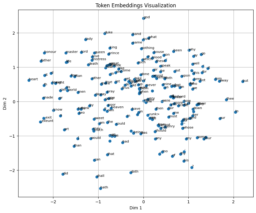
The visualization above shows only the first two dimensions of the embedding space. We can see several clusters including character names, royal titles, and tokens that follow apostrophes in words like ne’er, ’tis and o’er. This shows that the JEPA model is learning informative embeddings.
We can also observe what words are closest in embedding space.
def neighbour_table_l2(words, n=5):
    device = next(encoder.parameters()).device
    encoder.eval()

    vocab_ids = torch.arange(len(vocab)).to(device)

    with torch.no_grad():
        vocab_emb = encoder(vocab_ids)

    rows = []

    word_order = {w: i for i, w in enumerate(words)}

    for word in words:
        if word not in token_to_id:
            continue

        word_id = token_to_id[word]

        with torch.no_grad():
            query_emb = encoder(torch.tensor([word_id]).to(device))

            x_sq = (query_emb ** 2).sum(dim=1, keepdim=True)
            v_sq = (vocab_emb ** 2).sum(dim=1).unsqueeze(0)
            cross = torch.matmul(query_emb, vocab_emb.T)

            distances = (x_sq + v_sq - 2 * cross).squeeze(0)

            distances[word_id] = float("inf")

            top_ids = torch.topk(-distances, n).indices.tolist()

        for rank, i in enumerate(top_ids, 1):
            rows.append({
                "query": word,
                "query_order": word_order[word],
                "rank": rank,
                "token": id_to_token[i],
                "l2_distance": distances[i].item()
            })

    df = pd.DataFrame(rows)

    # enforce deterministic ordering for display
    df = df.sort_values(["query_order", "rank"])

    pivot_tokens = (
        df.pivot(index="query", columns="rank", values="token")
        .reindex(words)
    ).T

    display(pivot_tokens)

    return df


# ---- run ----
words = ["young", "king", "romeo"]
df = neighbour_table_l2(words, n=5)| query | young | king | romeo |
|---|---|---|---|
| rank | |||
| 1 | old | friar | malcolm |
| 2 | delicate | chief | hamlet |
| 3 | civil | tamora | wolsey |
| 4 | honourable | taking | lucius |
| 5 | troubled | perfect | viola |
It’s encouraging that “king” is near other professions, young is near other adjectives (including its opposite - old), and “romeo” is near other names.
As I mentioned earlier, it would be easy to extend this methodology to non-linear (e.g. MLP, CNN, RNN, Transformer) models and use larger contexts and targets than single words. It’s also possible to play around with other hyperparameters like SIGReg regularizer coefficient, embedding dimension, and hidden dimension and try larger datasets.
Compared to many prior methods for getting word embeddings, this does appear to be less complicated than things like negative sampling (e.g. word2vec).
There’s also recent work on approximations to SIGReg that are likely more computationally efficient with very little downside (Akbar 2026).